Deep Reinforcement and InfoMax Learning
Published:
Link to poster: link
Recent advances in the area of self-supervised learning on pixel data (e.g. DIM, ST-DIM, CPC, MoCo, SIMPLE, BYOL) motivate the application of similar techniques in reinforcement learning.
A number of recent papers (e.g. CURL, DrQ) suggest that data augmentation, coupled with the exponential moving average of the target encoder, is a good-enough way to improve the model’s performance on standard benchmarks in discrete and continuous control.
Our recent joint work with the Microsoft Research Montreal lab (link to paper: link) rather looks into the predictive capabilities of classic value-based models and how they can be enhanced. Specifically, suppose we are given an RL agent, which is placed in a given state $s_t$ at time $t$. Furthermore, suppose that this agent currently follows the policy $\pi$ (this can be relaxed further down). We are interested in thow the current state $s_t$ and current action $a_t$ are able to predict the next state $s_{t+1}$ under $\pi$. Even though $\pi$ might not be optimal, predicting the next state helps the model keep a relevant set of features through the entire task (i.g. some form of PSR).
The quantity which allows us to boost this state-action-next-state similarity is the mutual information between the coupling $(S_t,A_t)$ and $S_{t+1}$:
\[\mathcal{I}[S_t,A_t\mid\mid S_{t+1}]=\int_{s_{t+1},s_t,a_t} \log \frac{p(s_{t+1}\mid s_t,a_t)}{p(s_{t+1})}dP(s_{t+1},s_t,a_t)\]We noted that simply looking at the information between $S_t$ and $S_{t+1}$ was not sufficient to reliably estimate the next state $S_{t+1}$, since the policy was averaged out in the expression.
Of course, the above formulation only captures one-step transition dynamics, so we can further generalize it by trying to predict the $k^{th}$ state from the current state-action pair:
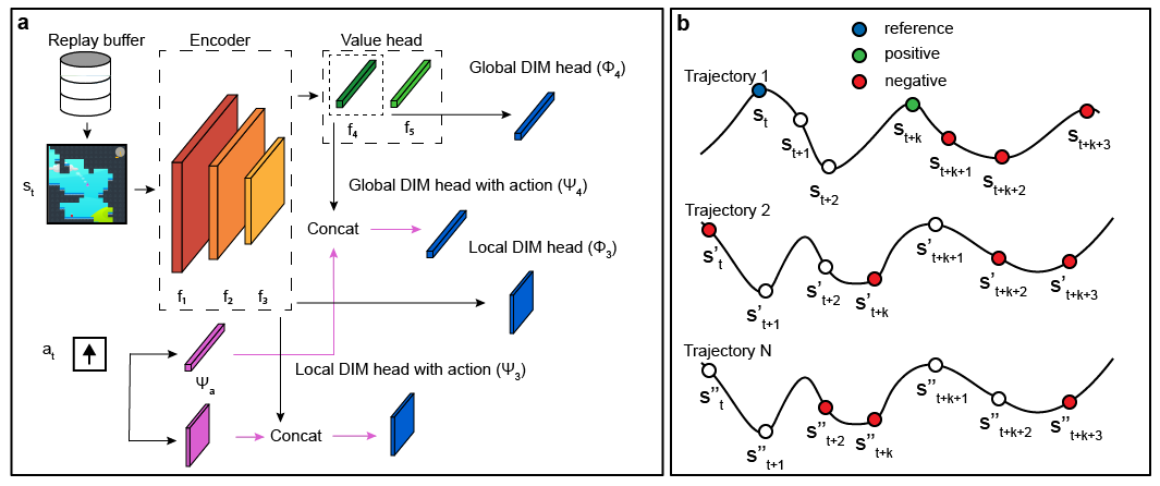
\[\mathcal{I}[S_t,A_t\mid\mid S_{t+k}]=\int_{s_{t+k},s_t,a_t} \log \frac{p(s_{t+k}\mid s_t,a_t)}{p(s_{t+k})}dP(s_{t+k},s_t,a_t),\;k>0\]The above quantity can be approximately measured by maximizing the infoNCE bound (van Oord, 2018), which requires to specify a distribution over positive and negative samples. In our case, to conserve the data efficency of off-policy algorithms, both distributions come from a randomly sampled batch of $(S_t,A_t,R_{t+1},S_{t+1},…,S_{t+k})$ tuples from the replay buffer. In fact, by performing a clever outer product along the batch dimension (pytorch code in paper), we are able to obtain an $n_{batch} \times n_{batch}$ similarity matrix, where the entry at position $(i,j)$ is equivalent to $\mathcal{I}[S_i,A_i\mid\mid S_j]$. The diagonal contains positive samples ($n_{batch}$ of them), while all off-diagonal entries ($n_{batch}(n_{batch}-1)$ of them) are taken to be negative samples.
The final model is inspired from AM-DIM, which maximizes the mutual information between different layers of the encoder (here, between conv layers and fc layers); it is schematically shown below.
Ising model
A classical example of a quasi-deterministic system is the Ising model on a 2-d lattice. The spin of each node can be set to either +1 or -1, depending on all 4 neighbor’s spins. The temperature parameter controls the rate at which the system evolves (high temperature typically means more movement in spins).
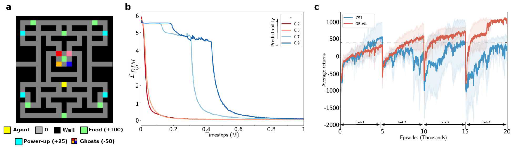
To assess whether DRIML can pick up this system, we let a $84\times 84$ lattice be sampled i.i.d. from a Rademacher(0.5) distribution. Then, a random $42\times 42$ portion of the lattice gets assigned an Ising model with $\beta=0.4$ being the inverse temperature. We fit DRIML to the $84\times 84$ screen, and show the results below.
| Ising model | DRIML scores |
|---|---|
 |  |
PacMan results
Since the auxiliary loss function does not have an explicit reward-boosting term, it is not expected to perform extremelly well on reward maximization tasks. However, the convolutions and fully-connected layers now have a notion of dynamics (i.e. how entities change with time) for environments on which samples we train the model on. Which is precisely why we tested the performance of a C51 agent augmented with our loss in a simple PacMan-style continual setting (see a). The agent is sequentially given access to 4 tasks, in each of which one of the four ghosts is deadly, but all four ghosts have identical transition dynamics.
It can be seen from the figure c below how the training rewards progress, as a function of training episodes, for the vanilla C51 agent, as well as for the C51 agent augmented with the infomax loss. Our loss forces the agent to keep track of all features predictive of next state, which is why it helps mitigate catastrophic forgetting in circumstances where the reward function can spontaneously change.
PacMan with quasi-deterministic noise injection
Optimizing the DRIML loss produces representations which are robust to quasi-deterministic changes that do not affect the behavior of the agent. To illustrate the difference between DRIML’s and C51’s invariance to such transformations, we conduct the following experiment: the 4 task PacMan setup from the previous section is overlaid on an Ising model with identical parameters as the ones in our paper. The Ising model sets pixels to either black (default wall color, -1 spin ) or purple (+1 spin) only in the walled regions of the maze, thus not affecting the behavior of the agent nor the ghosts. The systems evolves every timestep until termination of the episode, upon which the Ising model is reset to a new random configuration.
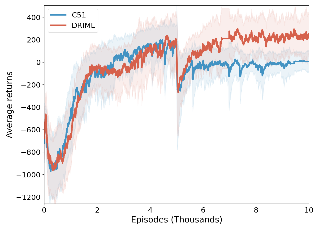
The figure above shows the moving average training performance of DRIML and C51 on two tasks with Ising noise injection in the walled areas. Note that not only does DRIML have a higher performance than C51, it also adapts more quickly to the change in tasks.
Procgen results
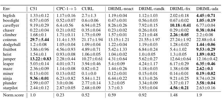
We also examined the performance of our model on the Procgen framework, where we let all agents train for 50M timesteps on 500 fixed levels, using only the DQN Nature encoder architecture (hence the reduced training setup). Training-time results are reported below.
Looking closer at the predictive timescale
The predictive timescale k has a very considerable impact on the performance of DRIML agents. In the table of results above, note the column called DRIML-randk. This corresponds to running DRIML-fix with a randomly sampled k (values can only be either 1 or 2, uniformly) for every row in the batch. The hypothesis was that if DRIML-randk works reasonably well, then randomization of the predictive timescale acts as a regularization, forcing the network to not only predict $s_{t+k}$, but also $k$ itself. However, this was not the case: DRIML-randk works okay-ish, but not near DRIML-ada’s performance.
Below, you can seen an ablation on both the batch-averaged proportion of actions taken by DRIML-ada, and the average $k$ over training steps (only for the most interesting games, the other 12 patterns were similar to either of these 4).
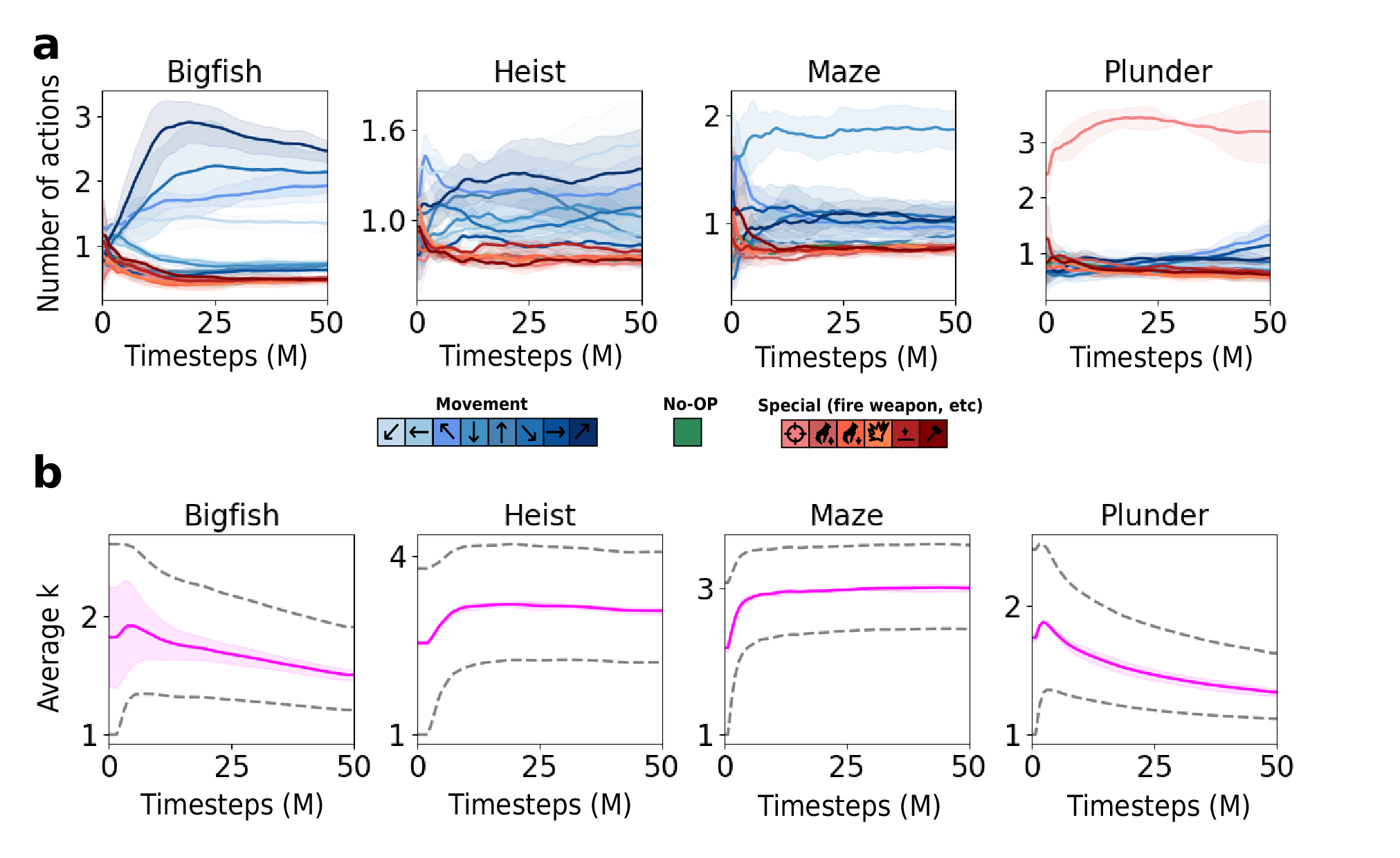
It’s interesting to see how shooting-based games, for example, tend to over-abuse of the firing action through the entire training process. This makes us think that $k$ should be picked based on the “expected novelty” in the state: if the agent repeats the same action 5 times and then abruptly switches to another one, chances are that something interesting happened at that switch, and DRIML should be able to predict this from pixels. Of course, this is rather hypothetical, but looking at the plot of $k$ over time, we clearly see that a trend is happening. Early values of $k$ (averaged over the batch), tend to be quite large, and progressively “cool down” to 1, which is very similar to an exploration-exploitation trade-off.
A side note on the non-homogeneous geometric sampling
We decided to select $k$ using a geometric distribution. We first learn the pairwise concordance of successive actions through a network $Q$, which is updated at the same rate as the main C51 network. Then, we store the predictions of $Q$ in a $\mathcal{A}\times\mathcal{A}$ row-stochastic matrix $A$.
When a batch of data comes in, we sample a Bernoulli variable $Z$ with probability $A_{a_1,a_2}$. If $Z=1$, $k$ is incremented by 1, and we repeat the process with $a_2,a_3$. This is very similar to sampling until a failure occurs, i.e. from a geometric distribution. Unlike the classical geometric distribution, here our success/failure probabilities change, which leads us to the non-homogeneous geometric (HNG) distribution.
The NHG distribution parametrized by $q_1,..,q_H$ has two neat properties:
It can represent any discrete distribution with positive support,
It’s mean is bounded from above and below by $\frac{1}{\max_i q_i} \leq \mathbb{E}[Z]\leq \frac{1}{\min_i q_I}$. So, in theory, by clipping the output of the network $Q$ to be between, say, $[\varepsilon,1-\varepsilon]$, we would guarantee that the average will be between $\frac{1}{1-\varepsilon}$ and $\frac{1}{\varepsilon}$.
So NHG is general enough that we are not loosing anything by adopting this form for $k$, and is very easy to sample from in an on-line fashion.
To cite:
@inproceedings{mazoure2020deep,
  title={Deep Reinforcement and InfoMax Learning},
  author={Mazoure, Bogdan and Combes, Remi Tachet des and Doan, Thang and Bachman, Philip and Hjelm, R Devon},
  journal={Advances in Neural Information Processing Systems},
  year={2020}
}